Mumbo 2 views, 2 classes example

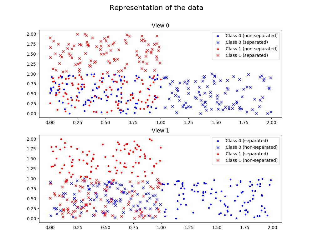
In this toy example, we generate data from two classes, split between two two-dimensional views.

For each view, the data are generated so that half of the points of each class are well separated in the plane, while the other half of the points are not separated and placed in the same area. We also insure that the points that are not separated in one view are well separated in the other view.

Thus, in the figure representing the data, the points represented by crosses (x) are well separated in view 0 while they are not separated in view 1, while the points represented by dots (.) are well separated in view 1 while they are not separated in view 0. In this figure, the blue symbols represent points of class 0, while red symbols represent points of class 1.

The MuMBo algorithm take adavantage of the complementarity of the two views to rightly classify the points.

• 
• 

Out:

After 3 iterations, the MuMBo classifier reaches exact classification for the
learning samples:
  - iteration 1, score: 0.75
  - iteration 2, score: 0.75
  - iteration 3, score: 1.0

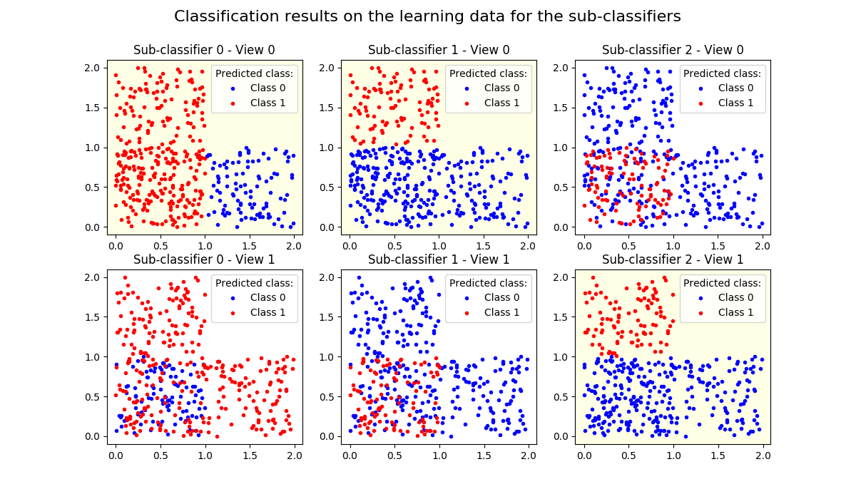
The resulting MuMBo classifier uses three sub-classifiers that are wheighted
using the following weights:
  estimator weights: [0.54930614 0.80471896 1.09861229]

The two first sub-classifiers use the data of view 0 to compute their
classification results, while the third one uses the data of view 1:
  best views: [0 0 1]

The first figure displays the data, splitting the representation between the
two views.

The second figure displays the classification results for the sub-classifiers
on the learning sample data.

/home/dominique/projets/ANR-Lives/scikit-multimodallearn/examples/mumbo/plot_mumbo_2_views_2_classes.py:127: UserWarning: Matplotlib is currently using agg, which is a non-GUI backend, so cannot show the figure.
  plt.show()

import numpy as np
from multimodal.boosting.mumbo import MumboClassifier
from matplotlib import pyplot as plt


def generate_data(n_samples, lim):
    """Generate random data in a rectangle"""
    lim = np.array(lim)
    n_features = lim.shape[0]
    data = np.random.random((n_samples, n_features))
    data = (lim[:, 1]-lim[:, 0]) * data + lim[:, 0]
    return data


seed = 12
np.random.seed(seed)

n_samples = 100

view_0 = np.concatenate((generate_data(n_samples, [[0., 1.], [0., 1.]]),
                         generate_data(n_samples, [[1., 2.], [0., 1.]]),
                         generate_data(n_samples, [[0., 1.], [0., 1.]]),
                         generate_data(n_samples, [[0., 1.], [1., 2.]])))

view_1 = np.concatenate((generate_data(n_samples, [[1., 2.], [0., 1.]]),
                         generate_data(n_samples, [[0., 1.], [0., 1.]]),
                         generate_data(n_samples, [[0., 1.], [1., 2.]]),
                         generate_data(n_samples, [[0., 1.], [0., 1.]])))

X = np.concatenate((view_0, view_1), axis=1)

y = np.zeros(4*n_samples, dtype=np.int64)
y[2*n_samples:] = 1

views_ind = np.array([0, 2, 4])

n_estimators = 3
clf = MumboClassifier(n_estimators=n_estimators)
clf.fit(X, y, views_ind)

print('\nAfter 3 iterations, the MuMBo classifier reaches exact '
      'classification for the\nlearning samples:')
for ind, score in enumerate(clf.staged_score(X, y)):
    print('  - iteration {}, score: {}'.format(ind + 1, score))


print('\nThe resulting MuMBo classifier uses three sub-classifiers that are '
      'wheighted\nusing the following weights:\n'
      '  estimator weights: {}'.format(clf.estimator_weights_))

print('\nThe two first sub-classifiers use the data of view 0 to compute '
      'their\nclassification results, while the third one uses the data of '
      'view 1:\n'
      '  best views: {}'. format(clf.best_views_))

print('\nThe first figure displays the data, splitting the representation '
      'between the\ntwo views.')

fig = plt.figure(figsize=(10., 8.))
fig.suptitle('Representation of the data', size=16)
for ind_view in range(2):
    ax = plt.subplot(2, 1, ind_view + 1)
    ax.set_title('View {}'.format(ind_view))
    ind_feature = ind_view * 2
    styles = ('.b', 'xb', '.r', 'xr')
    labels = ('non-separated', 'separated')
    for ind in range(4):
        ind_class = ind // 2
        label = labels[(ind + ind_view) % 2]
        ax.plot(X[n_samples*ind:n_samples*(ind+1), ind_feature],
                X[n_samples*ind:n_samples*(ind+1), ind_feature + 1],
                styles[ind],
                label='Class {} ({})'.format(ind_class, label))
    ax.legend()

print('\nThe second figure displays the classification results for the '
      'sub-classifiers\non the learning sample data.\n')

styles = ('.b', '.r')
fig = plt.figure(figsize=(12., 7.))
fig.suptitle('Classification results on the learning data for the '
             'sub-classifiers', size=16)
for ind_estimator in range(n_estimators):
    best_view = clf.best_views_[ind_estimator]
    y_pred = clf.estimators_[ind_estimator].predict(
        X[:, 2*best_view:2*best_view+2])
    background_color = (1.0, 1.0, 0.9)
    for ind_view in range(2):
        ax = plt.subplot(2, 3, ind_estimator + 3*ind_view + 1)
        if ind_view == best_view:
            ax.set_facecolor(background_color)
        ax.set_title(
            'Sub-classifier {} - View {}'.format(ind_estimator, ind_view))
        ind_feature = ind_view * 2
        for ind_class in range(2):
            ind_samples = (y_pred == ind_class)
            ax.plot(X[ind_samples, ind_feature],
                    X[ind_samples, ind_feature + 1],
                    styles[ind_class],
                    label='Class {}'.format(ind_class))
        ax.legend(title='Predicted class:')

plt.show()